Introducing datagoboop

datagoboop is an R package for data sonification, or the audio version of data visualization. This project started off while I was dreaming of representing data as a symphony — our ears can with some training pick out each instrument in a symphony orchestra (maybe 15-20 instruments), whereas representing more than 4 or 5 variables in one plot is usually quite chaotic.

I asked Sebastian Waz and Jaylen Lee to join me in putting together this first pass at an R package for data sonification. While we haven’t quite gotten to symphonic sound — turns out a library of high-quality audio files gets large fast, so most output from datagoboop sounds more like 8-bit video game music 😜 — we still think it sounds pretty neat!

Why datagoboop

There are a few other data sonification packages for R, such as

• sonify
• audiolyzr
• playitbyr

(audiolyzr in particular sounds pretty neat!)

The main difference between these packages and datagoboop is that datagoboop includes several built-in sonification versions of common plots, but also allows users to build audio plots piece by piece by providing a higher level of control and modular functions.

Setup

if (!requireNamespace("devtools")) install.packages('devtools')
devtools::install_github("akseong/datagoboop")

(You can also see the repo here)

Ground-level sonification

Pitch

Pitch in datagoboop is parameterized as idealized piano key numbers, where the pitch frequency (hz) is given as a function of the piano key number $n$ by $$f(n) = 2^{\big( \frac{n - 49}{12}\big)} \times 440$$

functions: cplay(), wplay()

To actually play audio, you’ll need to use either

• cplay(): audio playback with console controls (“control playback”)
• wplay(): audio playback better suited for .Rmd documents knitted to HTML.
  • in console, wplay() institutes a system timeout during playback.
    • use console controls instead: argument wplay_controls = TRUE
    • suppress playback completely: argument wplayback = FALSE
  • when knitting to html, wplay() saves the audio output as a .wav (named with timestamp), in a folder with the same name as your .Rmd file.

function: note()

library(datagoboop)

midC <- note(40)
wplay(
  midC, 
  file_path = "index.en.Rmark/midC.wav"
  )

note() is the most basic function in datagoboop — most other functions in datagoboop are built on top of it. The only required argument is a pkey (piano key); output is a .wav-format vector.

The optional arguments in note() are worth spending a moment on, since they appear frequently in datagoboop functions.

• optional arguments and defaults:
  • vol = 1, volume (values from 0 to 1);
  • dur = 1, duration in seconds;
  • fs = 44100, sampling rate (varies by speaker hardware/audio driver);
  • inst_lab = "sine", instrument type
    • "piano", "string", "wind", "bass", are built in, though as mentioned they sound like an 8-bit piano, string, flute, or bass
    • You can also add sounds using add_inst() if you don’t like our 8-bit sounds, then specify its label here;
  • decay = FALSE, exponential decay of sound;
  • decay_rate = 6, sound decay rate if decay = TRUE

midC_bounce <- note(
  pkey = 40, 
  vol = 1, 
  dur = 2, 
  inst_lab = "piano",
  decay = TRUE,
  decay_rate = 6
  )

wplay(
  midC_bounce, 
  file_path = "index.en.Rmark/midC_bounce.wav"
  )

functions: notes() & chords()

There is also a vectorized version notes() ….

pkeys <- 52:64      # piano keys for a 1 octave chromatic scale
vols <- 1:13 / 13   # increasing volume
durs <- 12:24 / 96  # slowing down

chrom <- notes(
  pkey = pkeys, 
  vol = vols, 
  dur = durs,
  decay = TRUE,
  progbar = FALSE
  )

wplay(
  chrom,
  file_path = "index.en.Rmark/chrom.wav"
  )

…. and a single chord function chord()

chord_prog <- c(
  chord(pkey = c(50, 54, 57), decay = TRUE), 
  chord(pkey = c(50, 55, 59), decay = TRUE), 
  chord(pkey = c(50, 54, 57), decay = TRUE), 
  chord(pkey = c(49, 55, 57), decay = TRUE), 
  chord(pkey = c(50, 54, 57), decay = TRUE)
)

wplay(
  chord_prog,
  file_path = "index.en.Rmark/chords.wav"
)

Example: audio histogram / violinplot

One of the first things we did after creating some of the basic playback functions was to try making an audio version of a histogram. A little modification turns it into something like a violinplot, which I think may convey the general shape a little more clearly.

This is pretty different from the built-in function sonify_hist() below, but the idea is to walk through construction of an audioplot using datagoboop’s ground-level functions.

Overall, we’re going to

1. x-axis $\mapsto$ pitch: map histogram breakpoints to pitch;
2. y-axis $\mapsto$ duration: map counts/bar heights to duration;
3. y-axis $\mapsto$ volume: scale volume to counts/bar heights.

I think it’s a bit clearer when we start off hearing the highest count bars, and then allow the lower count bars to gradually emerge (so we’ll do that 👍).

Audio Histogram

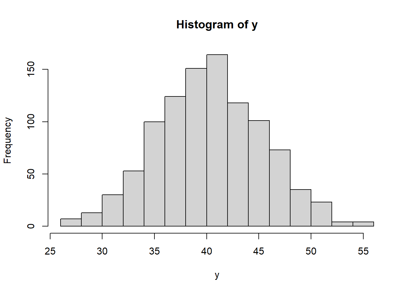
First, we generate the data, and create a histogram. We’ll specify the breaks manually (16 breaks = 15 bins), and also store the histogram’s info.

set.seed(2)
y <- rnorm(1000, 40, 5)
breaks = seq(
  floor(min(y)), 
  floor(max(y)) + 1, 
  length.out = 16
  )
hist_info <- hist(y, breaks = breaks)

Next, we’ll select a C-major scale to map the breaks to.

• major_scale() generates a vector of piano key numbers corresponding to a major scale starting at the specified tonic and number of octaves.
• The second line selects every other note in order to avoid dissonance. (There will still be some!)

Cmajor <- major_scale(tonic_pkey = 40, n_octaves = 4)
pkeys <- Cmajor[2 * 1:length(breaks)]

Now we need to construct each “bar” of the audio histogram — each bar gets a note. Some calculations are required, since we need to fill in each note with silence to start, then the pitch of the note for a duration that expresses bar height.

We use the sampling rate and desired total duration to calculate total length of each note (each note is a .wav vector, playable on its own).

fs <- 44100
total_dur <- 8
wave_length <- total_dur*fs

# scale the durations and volume to reflect counts
# i.e. the longest note is the bin with the highest counts
scaling <- hist_info$counts / max(hist_info$counts)
vols <- scaling + .25
durs <- scaling * total_dur
fill_durs <- wave_length - durs*fs

Last, we construct each note in a loop, and sum each note’s sound wave together to construct the audio histogram’s sound wave.

audiohist <- rep(0, wave_length)
for (i in 1:length(durs)){
  wave_i <- c(
    # notes begin with silence
    rep(0, fill_durs[i]),
    # audible portion of note 
    note(pkey = pkeys[i], 
         dur = durs[i], 
         vol = vols[i])
    )
  audiohist <- audiohist + wave_i[1:wave_length]
}

wplay(
  audiohist, 
  file_path = "index.en.Rmark/hist.wav"
  )

Audio Violinplot

I like the overall effect of the histogram — sort of like an island emerging out of the water. But the tails are very hard to hear. So, let’s try a violin plot, which we can do simply by reversing the sound vector and placing it back to back.

wplay(
  c(audiohist, rev(audiohist)), 
  file_path = "index.en.Rmark/violin.wav"
  )

(A small happy accident if you listen closely: around 5 seconds in, you can hear a progression in there that sounds — just for a moment — like the opening to Debussy’s La Fille Aux Cheveux De Lin)

function: sonify_hist()

datagoboop also has a built-in audio histogram function:

• counts/bar height $\mapsto$ pitch
• x-axis $\mapsto$ time
• static bursts mark quartiles

# requires dataframe as input
df <- data.frame(y)
wplay(
  sonify_hist(
    data = df, 
    var = "y", 
    breaks = 16, 
    duration = 5
    ),
  file_path = "index.en.Rmark/sonifyhist.wav"
  )

Next up: built-in audio plot analogues

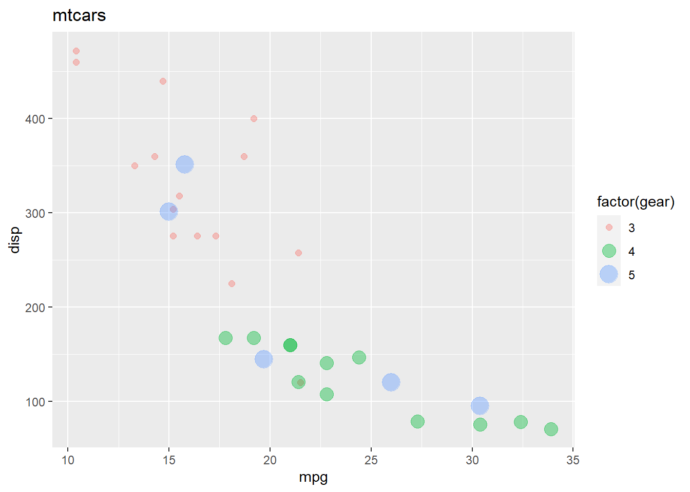
Next post will cover some of the basic plot types built-into datagoboop, for example, a scatterplot, in which the lower register indicates rising values in the $x$-variable, and the higher register indicates the value of the $y$-variable.

library(ggplot2)
ggplot(
  mtcars, 
  aes(
    y=disp, 
    x = mpg, 
    size = factor(gear),
    color = factor(gear)
    )
  ) + 
  geom_point(alpha = 0.4) + 
  labs(title = "mtcars")

mtcars_audio <- sonify_scatter(
  data = mtcars,
  x_var = "mpg",
  y_var = "disp",
  factor_var = "gear",
  volume = "gear",
  vol_scaling = "binned 3 exp 2"
  )
# output suppressed; shows progress bar in console

wplay(
  mtcars_audio, 
  file_path = "index.en.Rmark/mtc.wav"
  )

A small parting gift

bp2 <- bach()

wplay(
  bp2,
  file_path = "index.en.Rmark/bach.wav"
  )